How to Eliminate Impermanent Loss

 Generally, markets are efficient in that it isn't easy to make above-average returns day-trading, and most mutual funds underperform market-weighted ETFs. Yet historically, in various applications, options have been underpriced for decades. For example, asset return distributions were known to have fatter tails than the lognormal distribution back in the 1960s (see Benoit Mandelbrot ('62) or Eugene Fama (' 65)). Most option market makers, however, applied the basic Black-Scholes with a single volatility parameter, which underpriced out-of-the-money options. On a single day, October 19, 1987, the stock market fell 17%, which, using a Garch volatility estimate, was a 7.9 stdev event. From a Bayesian perspective, that did not imply a miracle but, rather, a misspecified model. Option market-makers soon adjusted their models for out-of-the-money puts and calls, ending decades of underpricing (20 years before NN Taleb's Black Swan introduced the concept of fat tails to the masses as if it were 1986).

Another example is convertible bonds, which are regular bonds that are convertible into stock at a fixed price, a bond plus an equity call option. The optionality was underpriced for decades. In the 1990s, a hedge fund that merely bought these bonds hedged the option's equity delta and bond duration and generated 2.0 Sharpes, which is exceptional for a zero-beta strategy. Eventually, in the early 2000s, investment bankers broke these up into bonds and options, allowing them to be priced separately. This isolation highlighted the option underpricing, and this market inefficiency went away. One could add Korean FX options that were underpriced in the 90s, and I'm sure there were many other cases.

So, there is precedent for a lot of money locked up in money-losing short convexity positions, as with liquidity providers (LPs) on automatic maker makers (AMMs). However, LP losses explain why AMM volume is still below its 2021 peak; transformative technologies do not stagnate for three years early in their existence unless something is really wrong. It's like how multi-level marketing scams like Amway have a viable business model relying on a steady stream of new dupes; they can persist, but it's not a growth industry.

The Target

The way to eliminate AMM LP convexity costs centers on this formula:

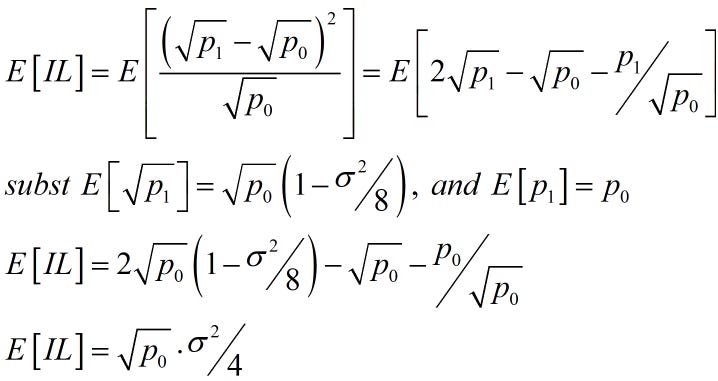
Impermanent Loss (IL) = LPvalue(pt) – HODL(pt)

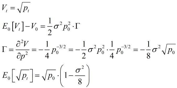
LPvalue(p_t) is the value of the LP position at the new price, p_t, and the 'hold on for dear life' (HODL) portfolio is the initial deposit of LP tokens valued at the new price. It turns out that this difference is not an arbitrary comparison but instead captures a fundamental aspect of the LP position, the cost of negative convexity in the LP position. The expected value of the IL is the LP's convexity cost, which is called theta decay in option markets.

The LP convexity cost also equals the expected value decay of a perfectly hedged LP position (minus fees). Hedging is often thought of as reducing IL, and it does reduce the variance of the IL, eliminating extreme LP losses. However, this does not affect the mean IL, which, over time, equals the expected value. Lowering a cost's variance reduces required capital, which is why hedging is a good thing, but it will not solve the IL’s main problem, its mean, which is generally larger than fees for significant capital-efficient pools.

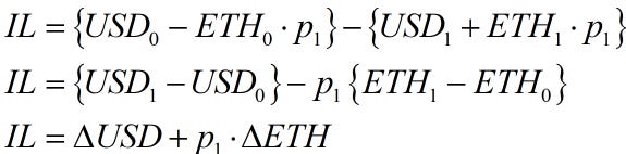
If we expand the above formula, we can rearrange variables to get the following identical equation as a function of pool token quantity changes and the current price (see here for a derivation).

IL = USDchange + pt×ETHchange

I am using a stablecoin USD and the crypto ETH as my two tokens because it makes it easier to intuit, though this generalizes to any pair of tokens (I like to think of prices in terms of dollars, not token A, but that's just me). The duration used to calculate the token changes implies the same LP hedging frequency. 24 hours is a pretty good frequency as hedge errors cancel out over a year via the law of large numbers, but anything between 6 hours and 1 week will generate similar numbers. If we can set ETHchange=0, USDchange will be near zero, and we will effectively eliminate IL.

An Extreme Base Case

One way to eliminate IL is to have a single LP who can trade for free while everyone else trades for a fee. Whenever the AMM price differs from the true price by less than the fee, only the LP can profit from arbitrage trading. A simple way to intuit this is to imagine if an AMM was created and not publicized, so it has no traders outside of the creator who assumes the role of LP and arbitrageur. With no other traders, he is trading with himself in a closed system. If his accounts are netted, he could both set the price on his contract efficiently and hedge his IL; nothing changes except the price. His net position in the tokens is static: ETHchange=0, IL=0.

It's helpful to think of traders as being two types: arbitrage and noise. Arbitrage traders are trying to make instant money off minor price discrepancies between exchanges; noise traders are like white noise, mean zero net demand that flows in like Brownian motion. A market price equilibrates supply and demand, so the volume that nets out is, by definition, noise. Noise traders are motivated by individual liquidity shocks, such as when a trader needs money to pay taxes, or the various random buy and sell signals generated by zero-alpha trading strategies.

If the AMM's base trading fee was 15 bps, and the LP could trade for free, the LP could turn loose an automated trading bot based on the Binance/CME/Coinbase price, trading whenever the mispricing exceeded 10 bps. Over time, the LP/arbitrager will be responsible for all the AMM's net price changes. With the AMM at the equilibrium price, immune to arbitrage by non-LP traders, the other trades will be white noise, net zero demand, by definition.

The figure below shows how the LP's ETH position for an AMM restricted range from $1300 to 1700 changes. The Pool ETH change implies traders are accumulating an offsetting amount; if the pool lost 2.5 ETH, traders gained 2.5 ETH. This net trader accumulation is arbitrage trading because it is not random, which is mean-zero over time. Gross trading will be greater due to noise trading, and in a healthy exchange, the noise traders will compensate the LP for his predictable IL over time.

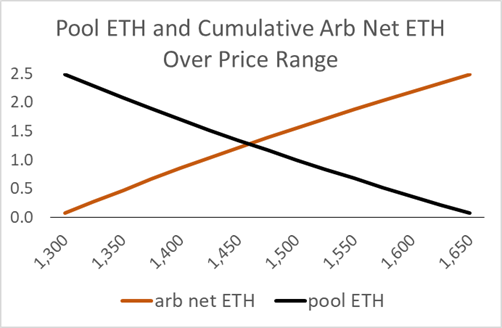
If the monopolist zero-fee LP were the arbitrageur, at any price his net ETH position would be the same; the sum of those lines, his net position on the contract, would be horizontal. With a constant net ETH position, his impermanent loss would be zero. This works because, unlike traditional markets, the option seller is not reacting to prices but setting them. The latency inherent in any decentralized AMM implies the price setter does not need any alpha, just an API to the lower latency centralized exchanges.

The LP would still have exposure to this net ETH position, but this is simple to hedge off the AMM with futures, as it would not need frequent adjusting.

If we add a separate margin account on the contract that held the LP's trades (with himself), they will net to a constant, his initial token position. The monopolist LP's net position on the contract would be represented as in the table below (on average).

Single LP with Exclusive Arbitrage Trading Access

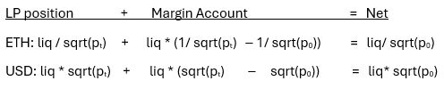
Thus, if the LP could trade for free, allowing him to dominate arbitrage, and he had a separate trading account on the contract, he could eliminate his IL without moving tokens on and off the blockchain or making other trades on different exchanges.

Multiple LPs

An AMM with only one LP would not work. An extensive set of LPs is needed to avoid centralization, which presents an attack surface for regulators and hackers; it is also needed to give the AMM unlimited scale. However, now we must consider LP competition. If we gave all the LPs free trading, a power law distribution of trading efficiency would invariably reveal a few dominant LPs monopolizing the arbitrage trading, shutting the slower LPs out and leaving them all exposed to IL as before.

Fortunately, the AMM provides a simple mechanism to allow all the LPs to arbitrage the price and hedge their positions simultaneously. This is because, on an AMM, the price is only changed by trades, so given a specific liquidity amount, a price change implies a specific change in ETH and vice versa. This makes it feasible to apply a rule using the LP's net ETH position on the contract to see if they qualify for the free discount.

Consider the following framework. Each LP gets a trading account in addition to their LP position. The key point is these accounts are netted, so like above, the LPs can retain a constant net position as the price moves significantly.

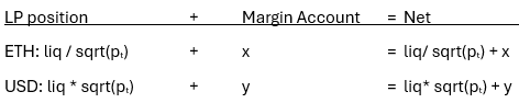
This can be adjusted to give them capital efficiency without changing the implications.[see footnote below] For my purpose in this post, this is irrelevant.

In the earlier example with one LP, his margin account's net change is calculated using the same liquidity as the pool because, with one LP, his liquidity is the pool's liquidity. This implied the LP's trades would always exactly offset his pool token changes. With many LPs, this is not so. A trade is against the entire pool, which is necessarily greater than any one LP. Thus, if LP(i) trades in a pool with many LPs, it will change LP(i)’s individual net position.

netETHchg(i) = (totLiq - liq(i))/totLiq *ETHtrade

As totLiq > liq(i), each trade changes the LP's net position, unlike when the monopolist LP trades with himself. For example, if an LP owns 10% of the liquidity, buying 1.0 token increases his margin position by 1.0 but decreases his pool position by only 0.1.

Assume LPs can only trade for free in the following conditions:

Buy for free only if

PoolEth(i) + MarginEth(i) - initEthDeposit(i) < + 0.01

Sell for free only if

PoolEth(i) + MarginEth(i) - initETHDeposit(i) >  - 0.01

If we assume the LP hedged his initial ETH deposit off-chain, the rules basically say if an LP is net net long, he cannot buy for free; if the LP is net net short, he cannot sell for free [presuming she hedged elsewhere initially, her ‘net net' position is her net position minus her initial deposit, as we assume it is hedged].

To see how this works, assume we have two LPs, Alice and Bob, with equal amounts of liquidity. Both Alice and Bob start with pool ETH positions of 990, and they have zero positions in their margin accounts. The trading fee is 0.5%, so all the price changes in this example are only profitable opportunities for Alice and Bob.

LP Pool, Margin, and Net ETH Balances

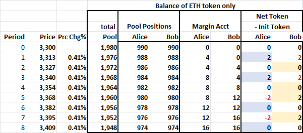
Assume the price initially rises by 0.41%, generating a arbitrage opportunity for the LPs. Alice wins the race and arbitrages this price discrepancy, setting the AMM price at its new equilibrium level of $3,313. She bought 4 ETH, and her pool position declined by 2 for a new ‘net net’ ETH position of +2. LP Bob just sees his pool position decline and has a new net net ETH position of -2; Bob is short, and Alice is long.

Alice cannot arb the AMM if the price rises again due to the rule preventing long LPs from buying at zero fee. If the price rises, Bob will win the arb race (by default), and LP’s Bob and Alice are each flat again. In the table above, Alice buys in the rows where she has a light blue box, and Bob buys in the rows where he has a light orange box. They can only buy when their net net position is flat or negative when prices are rising. This prevents Alice or Bob from dominating arbitrage.

If the price immediately went back down after Alice initially arbitraged the pool, only Alice could arbitrage the pool price. This is because in period 1, Alice is long, and Bob is short, so Bob cannot sell for free, while Alice can. When she does sell, she restores the initial net position for both herself and Bob. Alice’s extra trading is benign.

The LPs will experience net token position changes for single trades or small price movements. Over longer price movements, however, each individual LP's net token change would be insignificant, and assuming the LP hedged, their net net position would be insignificant.

There is no reason to pay arbs to set AMM prices, as the latency in decentralized blockchains implies arbitrage requires no special expertise, unlike the price discovery on the lowest latency exchanges. External arbitrageurs generate a deadweight loss for high-latency decentralized AMMs, so there is no trade-off with price efficiency.

A specialist with fast APIs and redundant arbitrage bot programs distributed in the cloud could manage a bot for a set of LPs. If the contract allowed LPs to whitelist another address that could do one thing on his account: trade for zero fee. The rule would prevent this arb vault manager from overtrading some accounts at the expense of others, as either it would single out one account for trades that cancel out, like in the case of Alice buying then selling above, or quickly find that her accounts that have traded first in one direction can no longer trade in that direction. One could cap trade size so the arb vault manager does not max out a trade on an LP to generate a profit for the other LPs. Competition among such specialists would allow passive LPs to get most of the benefit from arbitrage/hedging without creating and running their own arb bots.

It wouldn't work on coins not traded on major centralized exchanges because it presumes the true price is common knowledge. The next Shina Ibu will have to first trade on a conventional AMM. Yet, that's a minor amount of AMM volume.

Alternatives

As the equilibrium price is presumed to be on CEXes, and an equilibrium price implies net zero demand trading, one could use an oracle to update the AMM's last price to this price just as an LP arbitrage trade would. Over time, the LP net token changes would not be explicitly tied to price changes such that LP position values had negative convexity (i.e., linear in the square root of price). The main problem for oracle-based AMMs is centralization. This creates an attack surface for hackers. It also creates an attack surface for regulators, as the SEC knows where American Chainlink CEO Sergey Nazarov, for example, lives. Once they figure out how to do it—it took regulators several years to shut down InTrade—they will prevent his company from supporting anything that competes with regulated industries like finance and sports betting because regulation’s quid pro quo is protection from competition. Another problem is incentives, in that with more players with different actions, the state space complexity increases exponentially, so any solution will be more costly and less efficient. Arbitrageurs with more skin in the game would invest more time exploiting the oracle than the oracle would defending itself, especially as it requires a collective decision-making process and will be much slower to respond.

A decentralized limit order book (LOB) could avoid IL like an oracle-based AMM by allowing the LPs to move their resting limit orders costlessly to the latest CEX price, but there would be several problems. First, on-chain LOBs aspire to look and feel like the trading interfaces we are used to on centralized exchanges, so they emphasize low latency. Low latency leads to quasi, if not complete, centralization, an attack surface, and, more importantly, insiders who will get the equivalent of co-located server access. As third parties do not audit these ‘decentralized’ exchanges, the LOB leaders or a lower-level dev could sell undisclosed privileged access, and the costs would be virtually zero. It would take a lot of faith to presume they are immune to this subterfuge. Secondly, it would require many messages to cancel and replace resting limit orders. Unlike my mechanism, where one account rectifies the mispricing, on an LOB each LP account must be adjusted separately. On a CEX, these cancel-and-replace orders are costless, but if the blockchain is marginally decentralized, it will cost a few cents, and zero is a significant price point. Lastly, no one has presented a mechanism to incent a manager to oversee a set of LPs who wish to outsource their active management coherently. The LPs would still compete for favorable queue positioning, making it needlessly complicated and shutting out potential passive LPs.

The auction approach proposed by Maollemi et al. lets people bid to be the zero-fee trader. In that approach, the LPs would sell their right to fees to an arbitrageur who would get privileged zero-fee trading rights over some future period. The bidder pays a lump sum to the LPs, and the trading fees for that period go to the bid winner (meaning his trading fees return to him, so he trades for free). Assuming risk-neutrality and zero capital costs or other expenses, the arb would pay the expected arbitrage profit, which equals the expected LP convexity cost. They would also pay for the expected noise trader volume. Considering the arb bidder would be exposed to risk in that actual volatility and noise trader volume will be much lower than expected on occasion, he would pay considerably less than the expected value of the arbitrage opportunity and noise trading fees. The arb would have to hedge his trades on a different exchange, requiring extra collateral, and have to move tokens on and off the blockchain between those two exchanges (always losing one and gaining another). Lastly, frequent novel auctions can be manipulated, which means they will, especially at first.

Conclusion

The signature AMM is the ETH-USDC 5 bps pool on the Ethereum mainchain. Over the past 12 months, it has generated about $44MM in LP fee revenue and experienced $54MM in convexity costs. Yet even if LPs were, in aggregate, making a profit, the convexity cost is still significant and unnecessary. Given that the entire Uniswap AMM market is 4x the above pool, and there are other AMM protocols, that's several hundred million dollars a year wasted annually. The good news is this can be eliminated, propelling AMMs out of their doldrums and securing a long-term solution to an essential blockchain mechanism: swapping coins.

Most crypto people do not intuitively understand an LP's convexity costs, but they are not some new speculative theory (e.g., hedge fund sniping). Gamma, convexity costs, and theta decay have been analyzed empirically and theoretically for the past 50 years. They are the unavoidable consequence of convex payouts based on an exogenous underlying stochastic price. Constant product AMMs that link trade amounts to price changes, combined with the latency, allow the derivative owner (LP) to both hedge and set the underlying price simultaneously.

I haven't met anyone who understands this because they would be excited if they did. It's not often you find ways of saving hundreds of millions of dollars a year. My friends in academia or tradFi don't have much interest, let alone knowledge, of AMMs. My acquaintances in crypto, even those actively building AMMs, don't understand convexity beyond the technical definition, so they do not think it is a big deal. Fear of convexity costs is the beginning of AMM wisdom.

I wrote my dissertation in 1994 on low-vol stocks, noting they generated abnormal returns because they generate a slight premium to the market at 30% less risk (see here for a history of low-vol investing). I took a job as a bank risk manager but was busy pitching the idea to various asset managers, including several at the major investment banks. They didn't reject what I was saying but were always eager to know if well-known people or institutions in this field were on board. They weren't, and no one thought a fund offering virtually the same return as the SP500, regardless of risk, was compelling. I was out by the time low-vol investing started to grow. The responses I get from crypto people to this idea are similar.

It's not an abstract argument, just MBA-level finance. My best hope for this approach is that in a few years, LLMs will pick it up as they scrape the web for data, and via pure logic, over a couple of years, ChatGPT6 will use it as an answer for 'How do I remove impermanent loss?' There is pleasure in just being right about something important. 

footnote

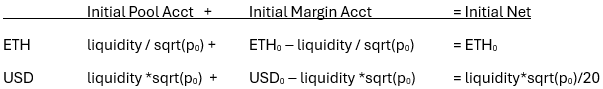
In a levered AMM, the initial pool amounts are multiples of the initial deposit. This implies the LP starts with debits in his margin account for both tokens. The process works as follows:

Take an initial ETH deposit, ETH₀. Given the initial price, p₀, and assuming a leverage of 20x, apply the following liquidity to that LP

liquidity = 20*sqrt(p₀)*ETH₀

Given that liquidity, the initial USD deposit, also levered 20 times, is calculated:

Initial USD deposit = liquidity*sqrt(p₀)/20

The objective of monitoring the LP’s net position for free trading is the same as above. Here, the initial margin account is negative, and the LP is susceptible to insolvency. However, a more pressing concern is whether the LP will be insolvent in one of the tokens, even though their total position value is positive. A pool where all the LPs are solvent, but the LPs have zero of one of the tokens would prevent purchases of that token. The solution is to allow liquidation based also on the minimum net position for the LP in the two tokens.

If the LP actively hedges its position, its net position will be constant in both tokens, so LPs would only be subject to liquidation if they exposed themselves to IL out of negligence. 

Spurious High Frequency Autocorrelation

 A curious aspect of high-frequency data is that most come from centralized limit order books (CLOBs) where the bid-ask spread makes the data look negatively autocorrelated as trades are randomly made at the bid and the ask.

The returns driving this pattern are well below transaction costs, so they do not generate an arbitrage opportunity. However, one might be tempted to use the high-frequency data to estimate variance for pricing options or convexity costs (aka impermanent loss, loss versus rebalancing). This is a problem because the 1-minute Gemini returns generate a variance estimate 40% higher than one derived from daily data.

Variance grows linearly over time; volatility grows with the square root of time. Thus for a standard stochastic process, the variance should be the same when divided by the frequency. If the return horizon is measured in minutes, the variance of the 5-minute return should be half of the variance of the 10-minute return, etc. Variance(ret(M minutes))/M should be constant for all M. It’s helpful to divide the data by a standard, which in my case is the variance of the 1-day return over this sample (1440 minutes), so we can clearly identify those frequencies where variance is over and under-estimated. If the ratio is above 1.0, this implies mean-reversion at this frequency (negative autocorrelation), and if below 1.0, this implies momentum (positive autocorrelation).

Here is the ratio of the m-minute return variance divided by m for various minutes, normalized by dividing by the 1-day return. It asymptotes to 1.0 at 300 minutes.

I added the ETH-USDC 5 and 30 bp pools, and we can see the effect of stasis created by the fee and lower transaction volume. The one-minute return variance ratios for AMMs are well below 1.0, implying momentum—positive autocorrelation—at that frequency. Again, the effect driving this is well below 5 basis points, so it’s not a pattern one can make money off.

A common and easy way to calculate variance is to grab the latest trade and update an exponentially weighted moving average. This would generate a variance estimate at an even higher frequency than once per minute. The perils of this are clear when many important data are linear in variance, such as the expected convexity cost, and 40% is big.

As a refresher, I show how the common concept for impermanent loss equaling a function linear in variance because it’s not obvious. We start with the original IL definition

This is measured as

The following AMM formulas can substitute liquidity and prices into the above equation.

plugging these in, we can derive the following formula.

This ‘difference in the square roots squared’ function calculates a realized IL over a period (from 0 to 1). If one estimated this using daily data over several months, it would equal the expected IL via the law of large numbers.

One can estimate the expected IL using the expected variance and gamma of the position. The key nonlinear function on the AMM LP position is the square root of price, which has negative convexity. This implies a simple variance adjustment to the current square root to get the expected future square root.

Note that in the above, the variance is for the time period from 0 to t, so if it’s an annualized variance applied to daily data, you would divide it by 365. Returning to the above IL formulated as a function of square roots, we can substitute for E[sqrt(p₁)] to see how this equals the ‘LVR’ equation with the variance.

Using (p₁/p₀ - 1)² for the variance will generate the same formula as the difference in square roots squared if you use the same prices. We can’t measure expected returns, but average returns equal expected returns over time, and that’s all we have. One chooses some frequency to estimate the IL, regardless of the method. Just be careful not to use returns under a 300-minute horizon, as these will bias your estimate. 

Moallemi's Auction-Managed AMM

A recent paper by Columbia professor Ciamac Moallemi and three Uniswap affiliates (Adams, Reynolds, and Robinson) presents a mechanism for recapturing the convexity costs. It builds upon Moallemi's previous work on automated market makers (AMMs) and arbitrage profit, published a year ago, which Moallemi presented at a16z crypto last summer. In that talk, he mentioned auctions as a way to reduce adverse selection costs for liquidity providers (LP).

AMMs' big problem is that LPs generally lose money in their popular capital-efficient (v3) pools. An LP's net profitability consists of revenue in the form of fee income and convexity.

LP profits = volume*fee – convexity costs

The LPs present traders with an option, and like all options, these are costly for the sellers. LP convexity costs have three mathematically equivalent formulations, and I posted three equivalent ways on Monday. Many only consider LP fee revenue as if convexity costs are just an academic hypothetical relative to an ideal. However, unlike the hedge fund sniping expense, option expenses are real, as reflected in standard option premiums above intrinsic value.

More relevant to this post, the convexity cost in an AMM is determined by two variables: the variance of the asset, which is exogenous to the AMM, and the liquidity in the AMM pool, which is endogenous. Both have a direct, linear impact on convexity costs.

AMM convexity costs = liquidity * sqrt(p₀) * variance / 4

The expected value of this formula is unaffected by the granularity of the data used to generate the variance, highlighting that this cost has nothing to do with the frequency of blocks, trading, or hedging. The convexity cost is the inverse of the gross arbitrage profit (noted in my Monday post), which is the profit to the arbitrageur collective pre-fees. 

The largest AMM on blockchains is the ETH-USDC 5 basis point v3 pool, which processes hundreds of millions of USDC daily. This year, the 5 bp pool is actually making money because its liquidity is down about 60%, which has a first-order effect on convexity costs. For example, last year, their liquidity was usually around 30MM, which implies a $100k trade would generate slippage of only 0.01%; currently, liquidity is around 10MM, so the slippage would be 0.04%. I don't think traders mind, as this is still far better liquidity than anywhere else. This LP profitability could be temporary, but this pool has not had this low level of liquidity for three months since 2021, suggesting LPs have wizened up. With only $150MM in capital in the pool, this annualizes to an excellent 10% annualized return. 

Average Daily Stats for ETH-USDC 5bp Uniswap v3 Pool

Unfortunately, this year's ETH-USDC 5bp pool performance is not typical, and regardless, addressing LP convexity costs is important. The larger capital efficient restricted range (v3) pool LPs lose money. Since January 1, 2023, the ETH-USDC 5bp pool has lost an average of $6k a day net, including $142k in fee revenue and $148k in convexity costs. If one could reduce these costs by a mere 10%, the pool LPs would be profitable.

The auction mechanism is presented formally per Moallemi's previous work, but the gist is straightforward. Arbitrageurs bid for the right to be the 'pool manager' who gets all fee revenue and sets the pool fee in a future period (e.g., a day). As they get all the fees paid, the pool manager will effectively trade for free because the fees come back to him as revenue, while other arbitrageurs would pay the X bp fee. This gives the pool manager a competitive advantage in arbitraging the pool, as those paying the fee will find any mispricing less than the fee unprofitable, while the pool manager could capture it. If the pool manager pays the expected fees and just half of the arbitrage revenue, virtually all v3 pool LPs would be profitable. This is because gross arbitrage revenue—i.e., excluding fees—is the flip side of their convexity costs.

Chicago professor Eric Brudish has been promoting frequent batch auctions as an alternative to CLOBs for the past decade (see here and here), highlighting the tax generated by hedge fund sniping, where speedy high-frequency traders scoop up resting limit orders before the hapless market makers can remove them. Milionis, Moamelli, Roughgarden, and Zhang's Loss vs. Rebalancing paper alludes to hedge fund sniping in the context of AMMs, but that's far-fetched. AMMs do not have race conditions analogous to traders picking off stale limit orders. Even within the snail's pace of blockchains, you do not see LPs trying to do the inverse of just-in-time liquidity to get out of the way of trades (removing liquidity before a big trade and then adding it back in after the trade). The sniping form of adverse selection is sexy, focusing on unsympathetic high-frequency traders portrayed by best-selling author and SBF fanboy Michael Lewis. Still, it's, at best, a curiosity. A generous estimation of its effect is 0.4 basis points on average CLOB stock market spread of 3.5 basis points—a trivial effect—and irrelevant in AMMs. The bottom line is that arbitrage profits generate standard adverse selection costs for all market makers. With AMMs, this cost has an explicit formula.

Nonetheless, the sniping-motivated auction literature explains why Professor Moamelli had an auction solution ready. Academics like auctions because, in theory, they do not have any deadweight losses and are efficient given simplifying assumptions. In practice, however, auction complexity generates problems, which is why most asset markets use CLOBs, which have reduced stock trading costs by 90% from 1990 through 2010.

Uncertainties in the Bidder's Expected Arbitrage Profit

Expected arbitrage profits are a linear function of variance, the square of volatility. The average daily variance using minute-downsampled data is 15 basis points, but the distribution is flat with a long tail, so we should expect bidders to assume something well below the mean.

Expected arbitrage profit is also a linear function of liquidity, which is also variable, especially in the popular v3 pools [they acknowledge their mathematical model only applies to v2 pools, but clearly, the application would be to v3 pools]. An intriguing example occurred on March 6, where the ETH-USDC 30 basis point pool liquidity was a whopping 30 times higher than its standard value over a 5% price interval, from $3,612 to $3,812. This was due to a massive LP position above the current price, where the LP probably thought it would be an excellent place to sell their ETH without any hassle. Interestingly, in this case, the LP lost $2.6MM in convexity costs and captured $2.2MM in fees, for a net loss of about 40 basis points on the $100MM in ETH they effectively sold. This was not a good deal, but not horrible given the size. The bottom line is that the expected variance of arb profit in the face of these liquidity spikes increases the expected arb profit volatility even more, making it more difficult because the LPs can withdraw it at any time.

Huge LP Position Taken Out Last Week

New Gaming Strategies

There is also the issue of the unknown unknowns in this setup. For example, in March 2020, a bidder rigged an auction to buy $8.32 million in ETH for zero DAI.  While that attack has been exposed, who knows what strategies this approach generates? For example, one could handicap an arbitrageur by withdrawing all of your liquidity when an adversary wins the pool manager's right. This could be a part of a long game where the punisher is willing to incur a cost to inflict a cost on others, getting them to stop bidding. As withdrawals are standard in v3 pools, it is difficult to see how to lock in liquidity and avoid this.

While the pool manager would have an advantage in arbitrage trading, they would not prevent noise traders from inadvertently taking some of their profit, as people will randomly buy when the AMM price is low. To prevent that, a pool manager might target traders using high latency front ends like Uniswap, and front-run these trades. Conversely, traders could see the current mispricing and anticipate an arbitrage trade, sandwich attacking the arbitrageur. While chains without the slow ETH mainchain could avoid explicit MEV tactics, one can expect motivated traders to see these transactions and get in front of them regardless, as latency for a decentralized blockchain is orders of magnitude greater than anything on centralized exchanges (100s of milliseconds vs 100s of microseconds). Unlike co-location on centralized exchanges, there would be back-room deals for access to the sequencers or RPC nodes, creating a deadweight loss to users.

Even without front-running, there is the question of how much of the total arbitrage profit a zero-cost ab could capture. These uncertainties would incentivize the Bidder to price arbitrage profit well below its expected value.

The paper also acknowledges the potential for an increase in sandwich attacks because the zero fee would make these more attractive. This would be like the front-running attack on lucky noise traders, but instead, it would target any large trade. The authors mention that off-chain auctions or private relays could address this, but this complicates the mechanism even further (how are private relays incented?). A strategy space grows exponentially in the number of moves players can make. Simplicity is the key to security.

Lastly, there is the issue of to what extent arbitrageurs are hedging off the blockchain. Given the mispricing distribution, we can see that the AMM price is generally within the fee for the 5 bp pool. As centralized exchanges charge at least 2.5bps, and there is always slippage (i.e., price impact, spread), the total cost of a hedge is at least 5 bps at the size they would trade (chunks of $50k). The arbs cannot hedge each AMM arbitrage trade with a CEX trade and lock in a profit. They probably hedge every hour or day or when their on-chain position reaches some absolute level. 

This practical nature of hedging implies the arbs will have the opposite risk profile as the LPs, becoming short during price declines and long on the opposite. As this arb would have tens of millions at work, it creates an endogenous risk amplification mechanism because a price decline would make the arb profit and also increase his short position, so he would have the means and motive to push it down further to hit stop-loss orders on centralized exchanges.

If average convexity costs for a pool were 100, the uncertainty about future liquidity and variance and how much of the arb could be captured would lower the didder's price well below that, say, half. The arb would have to pay hedging costs and gas fees, reducing this further. Then there is the loss of the fees the current arbs pay. It's possible that LPs would make less money, just as ObamaCare, in theory, was supposed to reduce medical costs but, in practice, increased them. 

Nevertheless, this is a step in the right direction, addressing a major problem in the status quo. Given that the difference between revenues and costs on these pools is 3%, the bidder could pay a mere 10% of the expected total arbitrage profits and bring LPs back to profitability. The biggest downside is that there are many complexities generated by this approach, implying a lot of work for a temporary solution, as the best-case scenario would capture a small fraction of the arbitrage profits, leaving significant room for improvement. 

LvR, Impermanent Loss, Theta, and Arbitrage Profits

Columbia professor Ciamac Moallemi, Uniswap's Adams, Reynolds, and Dan Robinson released a paper last week on recapturing some of the LP convexity costs by having the arbitrageurs bid for the right to trade at a reduced rate. I wanted to dive into that, but I thought it would be helpful to see how arbitrage profits relate to LP convexity costs, as this is not obvious. Further, people in this space use different terms and formulas for what I am calling the LP convexity costs, and it would be useful to clarify how they differ.

Ultimately, loss vs. rebalancing (LvR), impermanent loss (IL), convexity costs, and theta, represent the same thing. The estimation method for these metrics will use daily data generating random errors that become irrelevant due to the Law of Large Numbers. That is, resetting the IL benchmark each day is like hedging once a day or using daily data to estimate variance.

Impermanent Loss

The OG term for the peculiar LP cost in constant product AMMs is 'impermanent loss.' It was called that because while an LP could have a loss relative to their initial LP position, they would not lose money if the price moved back, implying that loss was not permanent. One could say that about any mark-to-market loss, but whatever, it's a commonly used term, and generally, people know what it means.

The basic idea was to compare the LP's current pool position with the original LP token deposit, though one can compare it to the prior tokens at any time in the past. I will use ETH and USDC as the tokens in my example, but the analysis generalizes to any tokens A and B, making it easier to intuit.

An LP position is necessarily adversely selected, losing ETH when the price rises gaining ETH when its price falls. It is this change in token quantities that drives the IL.

$\begin{array}{l}IL=Value(initialLPpositionatcurrentprice)-Value(LPatcurrentprice)\\ IL=\left\{US{D}_0-ET{H}_0\cdot p_1\right\}-\left\{US{D}_1+ET{H}_1\cdot p_1\right\}\\ IL=\left\{US{D}_1-US{D}_0\right\}-p_1\left\{ET{H}_1-ET{H}_0\right\}\end{array}$

This simplifies to a net token change valued at the ending price

Equation (1) - net LP token change: $IL=\Delta USD+p_1\cdot \Delta ETH$

The AMM generates simple formulas for ΔETH and ΔUSD as a function of liquidity and price changes. Note these are the pool token changes, excluding fees.

$\begin{array}{l}\Delta ETH=liq\cdot \left(\raisebox{1ex}{$1$}\!\left/ \!\raisebox{-1ex}{$\sqrt{p_1}$}\right.-\raisebox{1ex}{$1$}\!\left/ \!\raisebox{-1ex}{$\sqrt{p_0}$}\right.\right)\\ \Delta USD=liq\cdot \left(\sqrt{p_1}-\sqrt{p_0}\right)\end{array}$

Plugging this in and doing algebra, we get a square-root function that, multiplied by liquidity, generates the second metric for the LP's convexity cost:

$\begin{array}{l}IL=liq\cdot \left(\sqrt{p_1}-\sqrt{p_0}\right)+p_1\cdot liq\cdot \left(\raisebox{1ex}{$1$}\!\left/ \!\raisebox{-1ex}{$\sqrt{p_1}$}\right.-\raisebox{1ex}{$1$}\!\left/ \!\raisebox{-1ex}{$\sqrt{p_0}$}\right.\right)\\ IL=liq\cdot \left(\sqrt{p_1}-\sqrt{p_0}+\sqrt{p_1}-\raisebox{1ex}{$p_1$}\!\left/ \!\raisebox{-1ex}{$\sqrt{p_0}$}\right.\right)\\ IL=liq\cdot \left(2\sqrt{p_1}-\sqrt{p_0}-\raisebox{1ex}{$p_1$}\!\left/ \!\raisebox{-1ex}{$\sqrt{p_0}$}\right.\right)\\ IL=liq\cdot \frac{\left(2\sqrt{p_0{p}_1}-p_0-p_1\right)}{\sqrt{p_0}}\end{array}$

equation (2) - square of square roots: $IL=-liq\cdot \frac{{\left(\sqrt{p_1}-\sqrt{p_0}\right)}^2}{\sqrt{p_0}}$

Arbitrage Profit

As the LP's IL is based on net tokens coming in, someone took the opposite side; if the LPs net +1 ETH and −4000 USDC, traders net +1 ETH and −4000 USDC. As the LPs always lose money, the trader collective always makes money pre-fees.

The arbitrage profit is how much the arb is traded times the price changes.

$ArbitragePnL=\Delta ETH\cdot \left(p_1-fillPrice\right)$

We have the ΔETH function noted above, so we need the AMM fill price. This is the geometric mean of the starting and ending price.

$\begin{array}{l}fillPrice=\frac{\Delta USD}{\Delta ETH}=\frac{liq\cdot \left(\sqrt{p_1}-\sqrt{p_0}\right)}{liq\cdot \left(\raisebox{1ex}{$1$}\!\left/ \!\raisebox{-1ex}{$\sqrt{p_1}$}\right.-\raisebox{1ex}{$1$}\!\left/ \!\raisebox{-1ex}{$\sqrt{p_0}$}\right.\right)}=\frac{\left(\sqrt{p_1}-\sqrt{p_0}\right)}{\left(\sqrt{p_1}-\sqrt{p_0}\right)}\cdot \frac{\left(\sqrt{p_1}-\sqrt{p_0}\right)}{\left(\raisebox{1ex}{$1$}\!\left/ \!\raisebox{-1ex}{$\sqrt{p_1}$}\right.-\raisebox{1ex}{$1$}\!\left/ \!\raisebox{-1ex}{$\sqrt{p_0}$}\right.\right)}\\ fillPrice=\frac{p_1+p_0-2\sqrt{p_1\cdot p_0}}{2-\raisebox{1ex}{$\sqrt{p_0}$}\!\left/ \!\raisebox{-1ex}{$\sqrt{p_1}$}\right.-\raisebox{1ex}{$\sqrt{p_1}$}\!\left/ \!\raisebox{-1ex}{$\sqrt{p_0}$}\right.}\\ fillPrice=\frac{\sqrt{p_1\cdot p_0}\cdot \left(\raisebox{1ex}{$\sqrt{p_1}$}\!\left/ \!\raisebox{-1ex}{$\sqrt{p_0}$}\right.+\raisebox{1ex}{$\sqrt{p_0}$}\!\left/ \!\raisebox{-1ex}{$\sqrt{p_1}$}\right.-2\right)}{\left(2-\raisebox{1ex}{$\sqrt{p_0}$}\!\left/ \!\raisebox{-1ex}{$\sqrt{p_1}$}\right.-\raisebox{1ex}{$\sqrt{p_1}$}\!\left/ \!\raisebox{-1ex}{$\sqrt{p_0}$}\right.\right)}\\ fillPrice=\sqrt{p_1\cdot p_0}\end{array}$

As the fill price is positive, I ignored the sign in the above algebra. Substituting the fill price and ETH delta formula into the original equation generates the negative of equation(2), the square root function above.

$$\begin{array}{l}ArbitragePnL=liq\cdot \left(\raisebox{1ex}{$1$}\!\left/ \!\raisebox{-1ex}{$\sqrt{p_1}$}\right.-\raisebox{1ex}{$1$}\!\left/ \!\raisebox{-1ex}{$\sqrt{p_0}$}\right.\right)\cdot \left(p_1-\sqrt{p_1{p}_0}\right)\\ ArbitragePnL=liq\cdot \left(\sqrt{p_1}-\raisebox{1ex}{$p_1$}\!\left/ \!\raisebox{-1ex}{$\sqrt{p_0}$}\right.-\sqrt{p_0}+\sqrt{p_1}\right)\\ ArbitragePnL=liq\cdot \left(2\sqrt{p_1}-\raisebox{1ex}{$p_1$}\!\left/ \!\raisebox{-1ex}{$\sqrt{p_0}$}\right.-\sqrt{p_0}\right)\\ ArbitragePnL=liq\cdot \frac{\left(2\sqrt{p_1\cdot p_0}-p_1-p_0\right)}{\sqrt{p_0}}\\ ArbitragePnL=liq\cdot \frac{{\left(\sqrt{p_1}-\sqrt{p_0}\right)}^2}{\sqrt{p_0}}\end{array}$$

Remember this arbitrage pnl number excludes fees, which are an expense to the arbitrageur. Looking at a net price movement over an interval will also include incidentally lucky noise traders instead of true arbitrageurs. However, the critical point is that we can see the fundamental symmetry of arbitrage revenue and an LP's convexity expense.

Delta Hedged LP PnL

The LP's position has a delta, or price risk, that can be hedged. We can apply this hedge to any frequency we want, where the complexity of handling more data offsets the benefit of more frequent hedging. Removing the delta generates a much more efficient estimate of an LP's pnl.

The initial LP position is just {ETH, USDC}, so it is long whatever amount of ETH they deposited. The LP can just eyeball his ETH position to determine his hedge amount.

Position = USD₀ + ETH₀*p₀

The delta for an LP position can be confirmed by doing the math:

$\frac{dValu{e}_{LP}}{\partial p}=delta=\Delta =\frac{liq}{\sqrt{p}}=ET{H}_{LP}$

If we look at the change in the hedged LP position over time and assume we are looking at the change in ETH and USD without fees, we see it goes back to eq(1), the value of the net token change:

$\begin{array}{l}netLP=LPposition+hedge\\ netL{P}_0=\left\{US{D}_0+ET{H}_0\cdot p_0\right\}-ET{H}_0\cdot p_0=US{D}_0\\ netL{P}_1=\left\{US{D}_1+ET{H}_1\cdot p_1\right\}-ET{H}_0\cdot p_1\\ pnl=L{P}_1-L{P}_0=\left\{US{D}_1+ET{H}_1\cdot p_1\right\}-ET{H}_0\cdot p_1-US{D}_0\\ pnl=\Delta USD+p_1\cdot \Delta ETH\end{array}$

Given this result, we can use the logic above to show that this is equivalent to the square of square roots formula. Thus, comparing an initial token position to an initial token position is the same as the net pnl for an LP position hedged at some earlier token position. It is a different way to think about impermanent loss.

Theta

Finally, the Black-Scholes approach uses theta, which equals the expected loss from convexity in equilibrium (profits = 0). In their proof, they create a riskless portfolio of an option and a synthetically replicated inverse of that option via a dynamic hedging strategy that targets the delta. Negative convexity generates an adverse delta change in the option, whether the price goes up or down, which generates losses for the hedged seller. If one rehedges frequently, the losses will be smaller, but there will be more of them, and on average, they generate the same expected return whether one rehedges daily or every second. A convex position's theta equals the position's gamma, or second derivative, times the underlying asset's variance, divided by 2.

$theta=-\frac{1}{2}gamma\cdot variance$

Here, the variance is scaled to whatever one's frequency is. For example, with daily data, one would take the annual variance divided by 365. Variance is linear in time, which is why people trade variance swaps and not volatility swaps. Fortunately, calculating gamma for AMMs from its primitive is simple, so it leads to the following:

$\begin{array}{l}LPvalu{e}_{LP}=2\cdot liquidity\cdot \sqrt{p}\\ \frac{dLPvalu{e}_{LP}}{\partial p}=delta=\Delta =\frac{liq}{\sqrt{p}}=ET{H}_{LP}\\ \frac{d^{2}LPvalu{e}_{LP}}{\partial p^2}=gamma=\Gamma =-\frac{liq}{2\cdot p^{1.5}}\\ theta=-\frac{1}{2}gamma\cdot variance=\frac{1}{2}\cdot \left(\frac{liq}{2\cdot p^{1.5}}\right)\cdot \left(p^2\cdot {\sigma }^2\right)\end{array}$

Simplifying, we get a function that uses a variance term:

Equation (3) -variance over 4: $theta=liq\cdot \frac{\sqrt{p}\cdot {\sigma }^2}{4}$

While AMMs, unlike option markets, do not have theta per se as there is no option premium to decay, it still captures the option cost for any short gamma position. This cost is a function of convexity, not the delta, so it presumes the position is delta-hedged.

The LvR function is identical to equation 3, though it looks different because the pool's market value is used to normalize it:

$\frac{theta}{LPvalue}=-\frac{{\sigma }^2}{8}$

This is a handy formula, as volatility per day for many coins is 5%; it generates a cost 3.125 basis points per day, a fun fact. In practice, however, we need to get the liquidity and price data anyway to get the market value we would apply this to anyway. Given the LP market value function

$LPvalue=2\cdot liq\cdot \sqrt{p}$

If we multiply variance/8 by the LP value, we get equation (3), the variance function for the LP's convexity cost.

Unfortunately, my math/stats skills are insufficient to prove equations 2 and 3 are the same, but they are (or at least 99% approximations of each other).

$liq\cdot \frac{{\left(\sqrt{p_1}-\sqrt{p_0}\right)}^2}{\sqrt{p_0}}\approx liq\cdot \frac{\sqrt{p_0}\cdot {\sigma }^2}{4}$

This gives us three ways to calculate IL. If we use the same starting and ending times, they should be the same. That is, the variance term should use the variance in the [0,1] interval, and the ΔETH and ΔUSDC should also use the [0, 1] interval.

$nettokenchange:\Delta US{D}_{0,1}+p_1\cdot \Delta ET{H}_{0,1}$

$squareofsquareroot:liq\cdot \frac{{\left(\sqrt{p_1}-\sqrt{p_0}\right)}^2}{\sqrt{p_0}}$

$varianceover4:liq\cdot \frac{\sqrt{p_0}\cdot {\sigma }_{0,1}^2}{4}$

These are all costs to the LP and need to be subtracted from the LP fees to get the LP's total profitability. However, in practice, the net token change data from Uniswap's 'swap' event logs includes fees, so one does not need the daily volume to generate the net LP pnl; removing the fees would take more work. Thus, we do not need to add fee revenue if we use the swap data to get the LP's net token changes.

$nettokenchangePnL:\Delta US{D}_{0,1}+p_1\cdot \Delta ET{H}_{0,1}$

For the other approaches, we can multiply the absolute value of the USDC traded by the fees to get LP revenue. While the fees are paid in whatever token is sold to the pool, using the numeraire is an efficient approximation.

$squareofsquarerootPnL:USDCvolumetraded\cdot fee-liq\cdot \frac{{\left(\sqrt{p_1}-\sqrt{p_0}\right)}^2}{\sqrt{p_0}}$

$varianceover4PnL:USDCvolumetraded\cdot fee-liq\cdot \frac{\sqrt{p_0}\cdot {\sigma }_{0,1}^2}{4}$

The nice thing about the net token change approach is that you can avoid the noise generated by the fact that liquidity is not constant, especially in restricted-range pools, where it can vary quite a bit over the day. Unless you calculate these data using each trade, any liquidity number you use will be approximate and generate noise in one's estimate. Thus, I prefer the net token change approach.

I estimated the daily pnl for a pool and used the day's price return squared for the variance number.

Uniswap ETH-USDC v2 pool on Ethereum Mainnet

1/1/23-3/5/24

Net token change pnl:             $7,231

Square root pnl:                       $7,152

Variance pnl:                           $7,097

As the standard deviation in this period was $12k, these estimates are in complete agreement. The correlation between the square root and variance metrics is 99.9%, while the token change pnl correlation with those two is around 99.6%

Impermanent Loss != LvR ?

For reasons I find irrelevant, Milionis, Moallemi, Roughgarden, and Zhang emphasize their LvR approach (the variance function) as superior to the square root function. First, they note that IL depends on the initial position, as it uses a squared term, so the magnitude is different for given starting prices.

$ImpermanentLoss=liq\cdot \frac{{\left(\sqrt{p_1}-\sqrt{p_0}\right)}^2}{\sqrt{p_0}}$

This is like saying the return on a stock that moved from 100 to 150 is different for someone who bought it at 50 and someone who bought it at 100: one made 100%, the other only 50% over that price increase. In practice, we apply consistent starting prices for the collective of those long and short, or all the LPs, which is intuitive and straightforward. It is like assuming they delta hedge once each period.

Another concern is that the square root function is noisier. Yet, one can apply any of these formulas at whatever frequency you want: by minute, hour, day. Using hourly data is a lot more work with negligible benefit. The errors generated will be normally distributed and diversify away in the same way regardless of one's approach. If you use daily data to generate variance or generate your square of square roots, you lose the information from the intra-period price spike, but when you have hundreds of daily observations, the benefits of greater granularity are trivial.

What you call the LP's convexity cost does not matter. What matters is you use something close to daily data intervals and eliminate the LP's delta risk, as all the above metrics do.